Thrust Model

The main propulsion system in Moonlander is modeled as a first-order dynamic system. The actual thrust force approaches the commanded thrust force exponentially, with a time constant representing the engine response delay.

Assumptions:

The engine cannot change its thrust force instantaneously. Instead, it behaves like a first-order system (PT1 / first-order lag) with time constant $\tau$ .

This model class is mathematically equivalent to:
- RC circuits
- Thermal inertia
- Motor spin-up dynamics
- Low-pass filters

Physical / System Formulation:

The rate of change of thrust force is proportional to the difference between commanded and actual thrust force:

\dot{F}_T \propto (F_{T,cmd}-F_T)

Introducing the proportionality constant $\frac{1}{\tau}$ :

\dot{F}_T = \frac{1}{\tau} (F_{T,cmd}-F_T)

Interpretation:

- $F_{T,cmd}$ : commanded thrust force [N]
- $F_T$ : actual thrust force [N]
- $\tau$ : engine response time / inertia [s]

Limiting cases:
- $\tau \rightarrow 0$ → instantaneous response
- Large $\tau$ → slow engine response

Discrete Form (from ODE)

Starting from:

\dot{F}_T = \frac{F_{T,cmd}-F_T}{\tau}

Assuming $F_{T,cmd}$ is constant over a timestep $\Delta t$ , the analytical solution becomes:

F_T(t+\Delta t) = F_T(t)e^{-\Delta t/\tau} + F_{T,cmd} (1-e^{-\Delta t/\tau})

Rearranged:

F_{T,k+1} = F_{T,k} + (1-e^{-\Delta t/\tau}) (F_{T,cmd,k}-F_{T,k})

Step-by-Step Solution of the Differential Equation

We solve the first-order ODE:

\dot{F}_T = \frac{F_{T,cmd}-F_T}{\tau}

Step 1: Rearrange

Bring the equation into standard linear form:

\dot{F}_T + \frac{1}{\tau}F_T = \frac{F_{T,cmd}}{\tau}

Denote:

a=\frac{1}{\tau}, \quad b=\frac{F_{T,cmd}}{\tau}

Step 2: Homogeneous Solution

Solve:

\dot{F}_{T,h} + aF_{T,h} = 0

Using exponential ansatz:

F_{T,h}(t) = Ce^{-at} = Ce^{-t/\tau}

Step 3: Particular Solution

Since the forcing term is constant, use: $F_{T,p}=k$ .

Substituting into the ODE:

0+ak=b \implies k=F_{T,cmd}

Step 4: General Solution

F_T(t) = F_{T,h}(t) + F_{T,p} = Ce^{-t/\tau} + F_{T,cmd}

Step 5: Apply Initial Condition

At $t=0$ , $F_T(0)=F_{T,0}$ :

F_{T,0} = C+F_{T,cmd} \implies C = F_{T,0}-F_{T,cmd}

Step 6: Evaluate at t + Δt

F_T(t+\Delta t) = (F_{T,0}-F_{T,cmd}) e^{-\Delta t/\tau} + F_{T,cmd}

Expanding using $F_{T,0}=F_T(t)$ :

F_T(t+\Delta t) = F_T(t)e^{-\Delta t/\tau} + F_{T,cmd} (1-e^{-\Delta t/\tau})

Step 7: Intuition

- The system always converges toward $F_{T,cmd}$ .
- The convergence speed is governed by $\tau$ .
- Smaller $\tau$ → faster response.
- Larger $\tau$ → slower response.

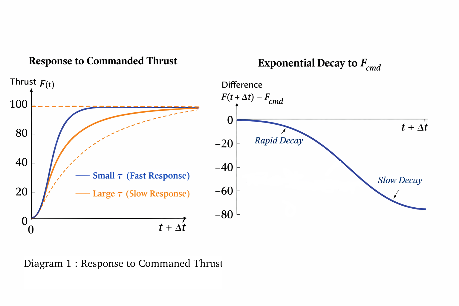
Illustration

The figure below shows the thrust force approaching the commanded target over time.

$Thrust response curve$

Fuel Consumption

The specific impulse is defined as:

I_{sp} = \frac{F_T}{\dot{m}g_0}

Where:
- $I_{sp}$ : specific impulse [s]
- $F_T$ : thrust force [N]
- $g_0 \approx 9.81$ : standard gravity [m/s²]

Solving for mass flow rate:

\dot{m} = \frac{F_T}{I_{sp}g_0}

Fuel mass decreases according to:

\dot{m}_f = - \frac{F_T}{I_{sp}g_0}

Typical values for common propulsion systems:

Engine Type	Fuel / Propellant	$I_{sp}\,[s]$
Liquid Rocket	LOX/LH2	450–465
Liquid Rocket	LOX/Kerosene	300–350
Solid Rocket	HTPB / Black Powder	200–300
Ion / Electric	Xenon, Hall / Electrostatic	1500–4000
Hybrid Rocket	HTPB + N₂O	250–300

Key Characteristics

First-order exponential response to commanded thrust force
Stable analytical discrete-time formulation
Real-time capable low-order propulsion model
Physically coupled fuel consumption
Suitable for guidance and control simulation
Numerically stable for variable simulation timesteps